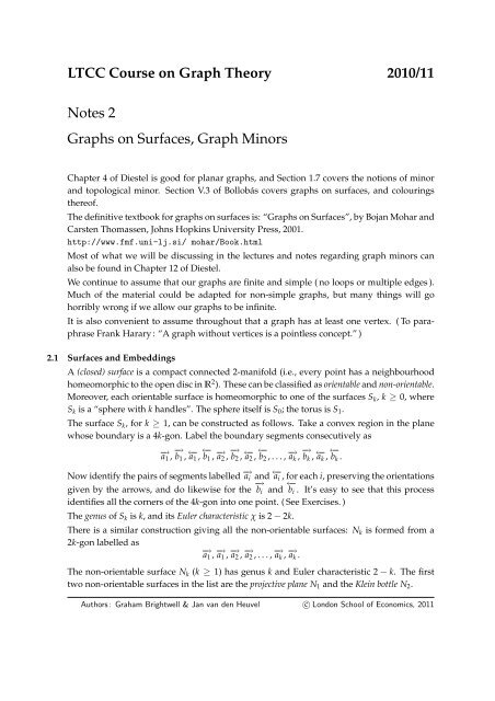
LTCC Course on Graph Theory 2010/11 Notes 2 Graphs on ...

<strong>LTCC</strong> <strong>Course</strong> on Graph Theory 2010/11 

Notes 2 

Graphs on Surfaces, Graph Minors 

Chapter 4 of Diestel is good for planar graphs, and Section 1.7 covers the notions of minor 

and topological minor. Section V.3 of Bollobás covers graphs on surfaces, and colourings 

thereof. 

The definitive textbook for graphs on surfaces is: “Graphs on Surfaces”, by Bojan Mohar and 

Carsten Thomassen, Johns Hopkins University Press, 2001. 

http://www.fmf.uni-lj.si/ mohar/Book.html 

Most of what we will be discussing in the lectures and notes regarding graph minors can 

also be found in Chapter 12 of Diestel. 

We continue to assume that our graphs are finite and simple ( no loops or multiple edges ). 

Much of the material could be adapted for non-simple graphs, but many things will go 

horribly wrong if we allow our graphs to be infinite. 

It is also convenient to assume throughout that a graph has at least one vertex. ( To paraphrase 

Frank Harary : “A graph without vertices is a pointless concept.” ) 

2.1 Surfaces and Embeddings 

A (closed) surface is a compact connected 2-manifold (i.e., every point has a neighbourhood 

homeomorphic to the open disc in R 2 ). These can be classified as orientable and non-orientable. 

Moreover, each orientable surface is homeomorphic to one of the surfaces S k , k ≥ 0, where 

S k is a “sphere with k handles”. The sphere itself is S 0 ; the torus is S 1 . 

The surface S k , for k ≥ 1, can be constructed as follows. Take a convex region in the plane 

whose boundary is a 4k-gon. Label the boundary segments consecutively as 

−→ a1 , −→ b 1 , ←− a 1 , ←− b 1 , −→ a 2 , −→ b 2 , ←− a 2 , ←− b 2 , . . . , −→ a k , −→ b k , ←− a k , ←− b k . 

Now identify the pairs of segments labelled −→ a i and ←− a i , for each i, preserving the orientations 

given by the arrows, and do likewise for the −→ b i and ←− b i . It’s easy to see that this process 

identifies all the corners of the 4k-gon into one point. ( See Exercises. ) 

The genus of S k is k, and its Euler characteristic χ is 2 − 2k. 

There is a similar construction giving all the non-orientable surfaces: N k is formed from a 

2k-gon labelled as 

−→ a1 , −→ a 1 , −→ a 2 , −→ a 2 , . . . , −→ a k , −→ a k . 

The non-orientable surface N k (k ≥ 1) has genus k and Euler characteristic 2 − k. The first 

two non-orientable surfaces in the list are the projective plane N 1 and the Klein bottle N 2 . 

Authors : Graham Brightwell & Jan van den Heuvel c○ London School of Economics, 2011

<strong>LTCC</strong> <strong>Course</strong> on Graph Theory Notes 2 — Page 2 

More details can be found in Bollobás, for instance. 

An embedding of a graph G = (V, E) in a surface S is a function taking each vertex x of G 

to a point ϕ(x) of S, and each edge xy of G to a Jordan curve in S, with endpoints ϕ(x) and 

ϕ(y), in such a way that the only intersections between the points and curves in the surface 

are those corresponding to incidences between edges and vertices of G. This all means what 

you think it ought to mean: this is exactly how we think of graphs being drawn on a surface. 

A graph can be embedded on the sphere S 0 if and only if it can be embedded on the plane, 

in which case it is called a planar graph. 

We’ll skip the work required to develop enough machinery to prove anything rigorously. 

( E.g., the “Jordan curve theorem” says that a closed Jordan curve in the plane has an inside 

and an outside, and it’s not easy to prove. ) The result we need is that, if we remove the 

image of G from the surface S, we are left with a number of connected components called 

the faces of the embedding. The embedding is a 2-cell embedding if each face is homeomorphic 

to the open unit disc. 

In the case of the sphere S 0 , the only way an embedding of a connected graph can fail to be a 

2-cell embedding is if the graph has no vertices. For surfaces with more interesting topology, 

this is a non-trivial condition. 

Two central questions of the subject are: (i) given a surface S, which graphs can be embedded 

on S (ii) given a graph embedded on S, what can we say about its chromatic number 

Of course, question (ii) includes the question of the chromatic number of planar graphs, 

covered in the previous lecture, as a special case. Here, we’ll concentrate on (i). 

2.2 The Euler-Poincaré Formula 

The Euler-Poincaré formula states that, if we have a 2-cell embedding of a graph on a surface 

S, then 

v − e + f = χ, 

where v is the number of vertices, e is the number of edges, f is the number of faces, and χ 

is the Euler characteristic of S. 

We’ll just prove this in the case where S is the plane, whose Euler characteristic is 2. 

Theorem 1 [Euler’s Formula] 

Let G be a connected graph with at least one vertex, embedded in the plane. Then v − e + f = 2, 

where v = |V(G)|, e = |E(G)|, and f is the number of faces of the embedding. 

Proof. We work by induction on the number f of faces. When f = 1, the graph has no cycles, 

so is a tree, and v = e + 1, which is consistent with the formula. 

For f ≥ 2, we suppose the result is true for embeddings with at most f − 1 faces, and take 

an embedding of a graph with f faces. Choose an edge separating two different faces, and 

delete it. The graph remains connected: the number of faces has decreased by one, as has the 

number of edges, while the number of vertices is unchanged. By the induction hypothesis, 

Euler’s formula holds for the new embedding. Thus it holds for our embedding. Thus, by 

induction, the formula is valid for all embeddings.


Euler’s formula is often quoted as referring to the number of vertices, edges and faces of a 

convex polyhedron in 3-space. The formula for polyehdra follows from the theorem for graphs, 

as a convex polyhedron can be “drawn in the plane” so that the notions of vertex, edge and 

face are preserved. 

Euler’s formula is often used in conjunction with a “double-counting” of the edges in an 

embedding. For i ≥ 3, let f i denote the number of faces of the embedding with i “sides”. 

Here we count sides in the natural way: for instance an embedding of an n-vertex tree yields 

one face with 2n − 2 sides. 

We note that ∑ i i f i counts the total number of sides of all the faces, and that each edge is 

counted exactly twice by this sum, so 

2e = ∑ i f i . 

i 

In particular we see that 2e ≥ 3 f , and using Euler’s formula now gives that e ≤ 3v − 6. 

Notice that this bound makes no mention of the embedding, so it gives a necessary condition 

for a graph to be planar. ( Indeed, the same argument gives an upper bound on the number 

of edges of a graph that can be embedded on any given surface. ) 

This means that the average degree of any planar graph is strictly less than 6, so that any 

planar graph contains a vertex of degree at most 5. Hence ch(G) ≤ 5 for any planar graph, 

which implies that χ(G) ≤ 6 – we saw last week that this can be improved! 

Today, we head in a different direction. From the above inequality, we see that a planar 

graph on 5 vertices has at most 9 edges, so the complete graph K 5 is not planar. Also the 

complete bipartite graph K 3,3 is not planar. To see this, notice that, in any embedding of a 

bipartite graph in a surface, all faces have an even number of sides, so in particular at least 4. 

Thus we have 2e = ∑ i i f i ≥ 4 f , and so e ≤ 2v − 4. 

2.3 Subgraphs and minors 

Now we know that K 5 and K 3,3 are not planar, we can deduce that any graphs “containing” 

them are not planar. For sure, this is true if our notion of containment is containment as a 

subgraph, but in fact we can make stronger statements by introducing more general notions 

of containment. 

• Let G be a graph. We define the following operations : 

* Removing a vertex means removing that vertex from the vertex set of G and also removing 

all edges that vertices is incident with from the edge set. 

* Removing an edge means removing that edge from the edge set of G. 

* Suppressing a vertex of degree two means removing that vertex and adding an edge between 

its two neighbours, provided that edge is not already present ( if the edge is already there, 

we don’t add a new one ). 

❍ ❍ u v w ✟ 

❍ ✟ 

❍ 

 

✲ ❍ ❍ u 

 

w ✟ 

❍ ✟ 

❍


* Contracting an edge : If e = xy is an edge of G, then contracting e means removing x and y, 

adding a new vertex z which is adjacent to all vertices that were adjacent to x or y, after 

which multiple edges are removed. 

• Let H and G be two graphs. 

❍ ❍ x e y ✟ ❍ ✟ 

❍ 

 

✲ ❍ ❍ z 

✟ 

❍ ✟ 

❍ 

 

 

* H is an induced subgraph of G, or G has H as an induced subgraph, notation H ≤ I G, if H can 

be obtained from G by a sequence of vertex removals. 

* H is a subgraph of G, or G has H as a subgraph, notation H ≤ S G, if H can be obtained 

from G by a sequence of vertex and edge removals. 

* H is a topological minor of G ( sometimes also called a topological subgraph or a subdivision ), 

or G has H as a topological minor, notation H ≤ T G, if H can be obtained from G by a 

sequence of vertex removals, edge removals, and suppression of vertices of degree two. 

* H is a minor of G, or G has H as a minor, notation H ≤ M G, if H can be obtained from G by 

a sequence of vertex removals, edge removals, and edge contractions. 

Note that in the definitions above we allow the sequences to have length zero, so every graph 

is a subgraph, etc., of itself. 

• There is a clear hierarchy of the order relations above : 

H ≤ I G =⇒ H ≤ S G =⇒ H ≤ T G =⇒ H ≤ M G. 

• The following useful result, whose proof is an exercise, gives an alternative characterisation 

of the minor relation. 

Theorem 2 

The following two statements are equivalent for all graph H, G : 

(a) H is a minor of G. 

(b) For each u ∈ V(H), there exists a subset V u ⊆ V(G) of vertices from G so that 

– the sets { V u | u ∈ V(H) } are disjoint, 

– each set V u , u ∈ V(H), induces a connected subgraph of G, and 

– for all u, v ∈ V(H) with uv ∈ E(H), there are vertices x ∈ V u and y ∈ V v with xy ∈ E(G). 

2.4 Minors and Embeddings 

Suppose that G is a planar graph, and that H is obtained from G by any of the operations 

of: vertex removal, edge removal, suppression of a vertex of degree 2, and edge contraction. 

We claim that H is also planar. 

The first two of these are obvious. For suppression of vertices of degree 2, we obtain an 

embedding of H by replacing the two Jordan curves representing the edges removed from G 

by a single Jordan curve representing the new edge of H. The same also holds if we replace 

“planar” by “embeddable on the surface S”, for any S.


For edge contraction, given an embedding of G, and an edge e = xy of G to be contracted, 

we derive an embedding of H by placing the new vertex z anywhere on the arc representing 

xy, and extending all the arcs incident with x or y inside thin tubes to reach z, following the 

path of the arc formerly representing xy. 

We then have the following consequence. 

Theorem 3 

If G can be embedded on a surface S, and G contains H as a minor, then H can be embedded on S. 

We say that the family of graphs that can be embedded on a surface S is minor-closed: if G is 

in the family, and H is a minor of G, then H is in the family. 

So certainly if G can be embedded on a surface, and G contains H in any of the other senses 

discussed above, then H can be embedded on the surface. 

Returning to the planar case, we now have the following results. 

Theorem 4 

(a) If G is planar, then G contains neither K 5 nor K 3,3 as a minor, 

(b) If G is planar, then G contains neither K 5 nor K 3,3 as a topological minor. 

2.5 Kuratowski’s Theorem 

Kuratowski’s Theorem says that the converses of both (a) and (b) in the previous theorem 

are true. 

Theorem 5 [Kuratowski’s Theorem] 

The following are equivalent. 

(a) G is planar; 

(b) G contains neither K 5 nor K 3,3 as a minor, 

(c) G contains neither K 5 nor K 3,3 as a topological minor. 

We’ve seen that (a) implies (b), and (b) implies (c) (since if G contains one of the graphs as a 

topological minor, it contains that graph as a minor). 

This section contains only a proof that (c) implies (b): if G contains one of K 5 or K 3,3 as a 

minor, then G contains one of K 5 or K 3,3 as a topoogical minor. 

The main part of the proof is that (b)/(c) implies (a). There is a relatively painless proof, 

due to Carsten Thomassen, in Diestel. Lemma 4.4.3 covers the case where G is 3-connected, 

which is the main part of the proof. 

Proof that (c) =⇒ (b). We use the characterisation of the graph minor relation given as Theorem 

2. 

Suppose first that G contains K 3,3 as a minor, and take a collection of six sets V h ⊆ V(G) as 

in Theorem 2. For each set V h , we identify three edges to V h from the sets V j , where j is in 

the opposite class of K 3,3 from h. These “land” at three, not necessarily distinct, vertices of 

V h : call these x, y, z. It isn’t hard to see that there is some vertex w h in V h (possibly equal to 

one or more of x, y, z) which has disjoint paths to x, y, z (possibly trivial) in G[V h ]. The six 

vertices w h , together with the various edges and paths, form a copy of a graph inside G that 

contains K 3,3 as a topological minor.


However – and hopefully this gives some insight into how and why the notions of minor 

and topological minor are different – if G contains K 5 as a minor then it need not contain K 5 

as a topological minor. Indeed, G can have a K 5 minor even if it has maximum degree 3, but 

a graph with a K 5 topological minor must have five vertices of degree 4. 

So one needs to prove that, if G contains K 5 as a minor, then it contains either K 5 or K 3,3 as 

a topological minor. Suppose then that there are five disjoint connected sets V a , V b , V c , V d , V e 

in G, with edges between each pair. The plan is to set off trying to find K 5 as a topological 

minor. So, for each V i , we find the four “landing points” x ij of edges from the other V j . Either 

there is a vertex w i in V i with four disjoint paths to the x ij , or there are two vertices f and 

g in V i , connected by a path, with two of the x ij sending paths to f and the other two to g, 

all five paths being internally disjoint. If this latter case occurs with any of the V i , then we 

change plans: in this case, we divide V i into two connected parts, one containing f and two 

of the x ij , and the other containing g and the other two x ij – the six vertex sets now witness 

that K 3,3 is also a minor, and therefore a topological minor, of G. 

2.6 Orderings and closedness of properties 

We will now leave the topic of graphs on surfaces, and examine the notions of graph containment 

for their own sake. To begin with, we observe that our relations of containment are 

all transitive (if G contains H and H contains J, then G contains J), and so give “orderings” 

on the set of all graphs: let us be more precise. 

If is a relation on a set X, then (X, ) is called a quasi-ordering or pre-order if the relation is 

reflexive ( x x for all x ∈ X ) and transitive ( (x y ∧ y z) ⇒ (x z) for all x, y, z ∈ X ). 

We say that a quasi-ordering (X, ) is without infinite descent if there is no infinite strictly 

decreasing sequence x 1 ≻ x 2 ≻ x 3 ≻ · · · ( where x ≻ y means y x and x ̸= y ). 

It is easy to see that the orderings defined in the previous section on the class G of all ( simple, 

finite ) graphs correspond to quasi-orderings without infinite descent. 

A subset A ⊆ X of a quasi-ordering (X, ) is an antichain if every two elements from A are 

incomparable ( i.e., if a, b ∈ A with a ̸= b, then a ̸ b and b ̸ a ). 

• Proposition 6 

If (X, ) is a quasi-ordering without infinite descent, then for every subset Y ⊆ X there is an 

antichain M ⊆ Y such that for all y ∈ Y there is an m ∈ M with m y. Such a set is called a set of 

minimal elements of Y. 

Note that the set of minimal elements need not be unique. If Y = {a, b} with a ̸= b, but both 

a b and b a, then both {a} and {b} are sets of minimal elements of Y. If we know the 

ordering (X, ) is a poset ( i.e., it is also anti-symmetric : (x y ∧ y x) ⇒ (x = y) for all 

x, y ∈ X ), then the set of minimal elements is always unique. 

• Let P be a property defined on the elements of X. We say that P is closed under or -closed 

if for every two elements x, y ∈ X we have that if x has property P and y x, then y also 

has property P. 

As an example, suppose property P is defined for G ∈ G as “G is bipartite”. This property 

is closed under both the subgraph and the induced subgraph ordering, but not under the


topological minor or the minor ordering. (See Exercises.) 

• Let (X, ) be a quasi-ordering and suppose P is a -closed property defined on the elements 

of X. Then we can talk about the set P of all elements in X that satisfy property P. And of 

course we also have the complement P = X \ P of all elements in X that do not satisfy 

property P. Let M be a set of minimal elements of P 

Since P is assumed to be -closed, we know that if x ∈ P and x y, then y ∈ P. This leads 

to the following crucial observation : 

x has property P ⇐⇒ there is no m ∈ M with m x. 

In other words : a property that is -closed is completely determined once we know a set of 

minimal elements of the set of elements that don’t have the property. Such a minimal set is 

called a minimal forbidden set of the property. 

• The observations above may provide a good description of certain properties and may provide 

efficient algorithms to test if a given element satisfies the property. This possible usefulness 

depends on the answers to questions like : Can we find a minimal forbidden set Is 

this set finite Is there a good algorithm to test if x y or not Etc. 

• You may wonder why we look at a set of minimal elements of the set P of elements in X that 

do not satisfy property P. Wouldn’t it be more natural to look at the set of maximal elements 

of P Yes, it would be more natural. But for the orderings we are considering such a set of 

maximal elements usually doesn’t exist. The orderings give natural minimal elements, since 

from every finite graph, we can only have a finite number of descending steps before we 

have to stop ( we’ve reached a graph with one vertex, say ). But in general we won’t have 

maximal elements ( except for very special properties ). 

• Here is an example illustrating the concepts above. 

For a graph G = (V, E), recall that the line graph L(G) = (V L , E L ) is the graph that has the 

edges of G as vertices : V L = E; and two edges are adjacent in the line graph if they have a 

common end-vertex in G. A graph H is a line graph if H ∼ = L(G) for some graph G. 

It’s easy to see that if H is a line graph, then every induced subgraph of H is also a line graph. 

Hence the property of “being a line graph”, defined on the set G of graphs, is closed under 

the induced subgraph ordering ≤ I . For this property, we actually do know the unique set of 

minimal forbidden elements.


Theorem 7 ( Beineke, 1968 ) 

A graph H is a line graph if and only if it does not contain one of the nine graphs below as an induced 

subgraph. 

2.7 Well-quasi-ordering 

• A quasi-ordering (X, ) is a well-quasi-ordering if for every infinite sequence x 1 , x 2 , . . . of 

elements from X, there are two indices i < j so that x i x j . 

Property 8 

The following two properties are equivalent for a quasi-ordering (X, ) : 

• (X, ) is a well-quasi-ordering; 

• (X, ) is a quasi-ordering without infinite descent and without infinite antichains. 

We’ll prove this in a later lecture. 

Requiring a quasi-ordering to be well-quasi-ordered is a very strong requirement. For instance, 

for the graph orderings defined in the first section, neither (G, ≤ I ), nor (G, ≤ S ), nor 

(G, ≤ T ), are well-quasi-orderings. For the induced subgraph ordering and the subgraph ordering, 

the sequence of cycles C 3 , C 4 , C 5 , . . . forms an infinite sequence that fails the condition 

in the definition. In one of the exercises you will be asked to find counterexamples yourself 

for the topological minor ordering. 

Although the whole class of graphs is not well-quasi-ordered under the topological minor 

ordering, some important subclasses are. 

Theorem 9 ( Kruskal, 1960 ) 

The class of all trees, with topological minor as the ordering, is well-quasi-ordered. 

• We are now able to give the main result regarding well-quasi-orderings. 

Property 10 

Let (X, ) be a well-quasi-ordering and P a -closed property on X. Then the minimal forbidden set 

of P is finite.


The importance of this property is that once we know that (X, ) is a well-quasi-ordering, 

then every property that is -closed has a finite minimal forbidden set. So if we also have 

an efficient way to test if two elements from X are related or not, then this way we would 

have efficient algorithms for every property that is -closed. 

2.8 Minors of graphs 

• Theorem 11 ( Robertson & Seymour, 1986–2004 ) 

The class of finite graphs is well-quasi-ordered under the minor ordering. 

More explicitly : for every infinite sequence G 1 , G 2 , . . . of graphs, there are indices i < j so that G i is 

a minor of G j . 

• Following the discussion from the previous section, Robertson & Seymour’s Theorem has 

the following consequence. 

Corollary 12 

Let P be a minor closed property of graphs. Then there exists a finite collection of graphs H 1 , . . . , H k 

so that for all graphs G we have 

G has property P ⇐⇒ G has none of H 1 , . . . , H k as a minor. 

• Since being embeddable on a given surface is minor closed, we get the following generalisation 

of Kuratowski’s Theorem for planar graphs. 

Corollary 13 

For every surface S there exists a finite set of graphs H 1 , . . . , H k , so that a graph G is embeddable on S 

if and only if G has none of H 1 , . . . , H k as a minor. 

For the sphere, we have seen that the forbidden minors are K 5 and K 3,3 . But even for the 

torus, the list of forbidden minors is not known completely. 

Exercises 

1 How does Euler’s formula for graphs embedded in the plane need to be modified to handle 

graphs with c components, where c is not necessarily equal to 1 

2 Consider the oriented surface S k , k ≥ 1. Draw a graph in S k by putting a vertex at each corner 

of the boundary 4k-gon, and an edge along each segment of the boundary, identifying any 

of these edges and vertices as necessary. Count the number of vertices, edges, and faces in 

this embedding, and verify the Euler-Poincaré-formula in this case. 

3 Describe the graphs not containing K 3 as a minor. Describe the graphs not containing the 

4-cycle C 4 as a minor.


4 Let P be the Petersen graph. ( If you don’t know what this is, find out! ) 

Show that P is non-planar: 

(a) using Euler’s formula; 

(b) by showing that P contains K 3,3 as a topological minor; 

(c) by showing that P contains K 5 as a minor. 

What is the minimum size of a set F of edges of P whose deletion leaves a planar graph 

5 Show that the property of being bipartite is not closed for the topological minor ordering on 

graphs. ( Very easy ) 

6 Prove that the property of having no connected component with more edges than vertices is 

minor-closed. Find as many minimal forbidden minors as you can for this property. 

7 Prove Theorem 2. 

8 Prove that the set of finite simple graphs G with the topological minor ordering ≤ T is not 

a well-quasi-ordering. In other words, give an infinite sequence of graphs G 1 , G 2 , . . ., for 

which there are no two indices i, j with i < j and G i ≤ T G j . 

( This is probably a hard question. Feel free to do an Internet search, but you must show that 

the sequence you give has the desired property. ) 

9 The first statement you are asked to prove in this question is an essential, but baby, step in 

the proof of Robertson & Seymour’s Minor Theorem. 

For a natural number n the n × n grid is the graph that has as vertices all pairs (i, j) with 

1 ≤ i, j ≤ n. And two pairs (i, j) and (i ′ , j ′ ) are adjacent if i = i ′ and |j − j ′ | = 1, or if j = j ′ 

and |i − i ′ | = 1. 

This is a sketch of the 4 × 4 grid : 

 

 

 

(a) 

 

Prove that every planar graph G is a minor of an n × n grid, for n large enough. 

( Hint : use Theorem 2. ) 

(b) Show that there exist planar graphs G that are not the topological minor of an n × n grid, 

no matter how large n is.

LTCC Course on Graph Theory 2010/11 Notes 2 Graphs on ...

You also want an ePaper? Increase the reach of your titles

Delete template?

Save as template?